Autoregressive Decoding: The Loop That Determines Your Serving Architecture
The core inference loop in an LLM is surprisingly small. Most implementations are only a few lines long: run a forward pass, sample the next token, append it to the sequence, and repeat.
I understood that mechanically for a while. What took longer to click was how many serving constraints come from that exact loop.
The pause before the first token and the latency between generated tokens are different bottlenecks. KV cache growth, batching behavior, throughput limits, and even why companies separate prefill and decode onto different GPU pools all trace back to the same property: generation is sequential.
Each token depends on the one before it.
This article walks through that idea from three levels: the transformer architecture, the implementation, and the production systems built around it.
Before you read this
This article has no hard prerequisites. It helps to know what a transformer is, but it is not required.
The KV cache article (read it here) goes one level deeper on what gets cached during inference and how it grows with sequence length. Read this one first if you are new to LLM serving.
How we got here: three architectures, one loop
If you have heard the word "transformer" and wondered what it actually means, this section is for you.
1. The original transformer (2017)
Picture a human translator working from French to English. First they read the entire French sentence. Then they write the English translation one word at a time, checking back against the original as they go.
The 2017 transformer architecture worked the same way. It had two halves:
8 Encoder: reads the input in parallel, all at once. Every word can attend to every other word simultaneously. Full bidirectional context.
- Decoder: writes the output one token at a time. Each new word can only look at what has been written so far, not at future words.
This made sense for translation. Encode the French sentence fully, then decode the English output word by word.
2. The interesting thing is that research went one way, industry went another!!
In 2018, two papers were released within months of each other. They made opposite bets on which half of the transformer mattered.
BERT threw away the decoder. It kept only the encoder, the part that reads everything at once with full bidirectional attention. The hypothesis: if you pretrain a deep bidirectional encoder on enough text, the representations it learns will transfer to almost any language understanding task. The hypothesis was correct. BERT dominated every NLU benchmark (GLUE, SQuAD, named entity recognition). For the next two years, virtually every NLP research paper was a BERT variant.
GPT threw away the encoder. It kept only the decoder, the part that generates one token at a time. OpenAI's hypothesis was different: if you train a model to predict the next token on enough text, at enough scale, you will eventually get a model that can do almost anything. GPT-3 (2020) and scaling laws (Kaplan et al., 2020) proved the bet. The decoder-only approach scaled cleanly: more parameters, more data, predictably better results, with no ceiling in sight.
Today, every major language model (GPT-4, Claude, Gemma, Llama) is decoder-only. The encoder half of the original transformer is not present.
3. Why decoder-only won for generation
The reason comes down to how training and inference match up. During training, a decoder-only model predicts the next token given all previous tokens. Left to right, always. During inference, it does exactly the same thing. There is no gap between training and deployment.
Encoder models cannot generate text naturally. Bidirectional attention requires seeing the full sequence. You cannot condition on partial output you have not generated yet. Encoder-decoder models can generate, but you carry two full model stacks in GPU memory instead of one, which matters when you are running at 70B+ parameters.
4. The attention mask that makes it sequential
The reason decoder-only models generate one token at a time comes down to one matrix. During training, the causal mask enforces that each token can only attend to previous tokens. During inference, that constraint holds. You cannot generate token n+1 until token n exists, because token n+1 attends to it.
Here is what each architecture looks like, what components it has and which direction attention flows:
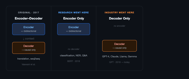 The original transformer architecture split into two directions after 2017. Research focused on encoder-only models like BERT for bidirectional language understanding, while production LLMs converged on decoder-only architectures because autoregressive next-token prediction scaled effectively for generation. Every major LLM today follows the decoder-only path.
The decoder-only architecture kept the piece that generates text and discarded the piece that reads it. That is the architecture running every major LLM today. The causal constraint is what makes generation sequential: each token can only look backward. Here is what that looks like at the token level:
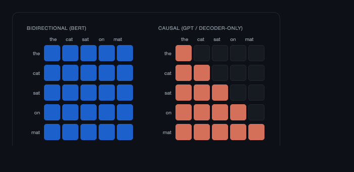 Bidirectional attention allows every token to attend to every other token. Decoder-only models use a causal attention mask that blocks future positions, forcing generation to proceed left-to-right one token at a time. The lower-triangular mask is the constraint that makes autoregressive decoding sequential.
Every red cell is an attention connection that exists. The dark cells are masked out. Token 3 ("sat") can attend to "the", "cat", and itself, but not to "on" or "mat". Token 5 ("mat") can attend to everything before it. The lower triangle is the constraint that makes generation sequential. You cannot compute row n until row n-1 is done, because row n depends on the token that row n-1 produced.
That is autoregressive decoding. One token at a time, strictly left to right, each token attending to all previous ones.
Level 1: The loop and what it forces
Every autoregressive language model generates text the same way. One token at a time. To produce token 10, the model runs a forward pass over tokens 1 through 9. To produce token 11, it runs a forward pass over tokens 1 through 10. Each step depends on all previous outputs. You cannot parallelize this.
That dependency is the constraint everything else flows from.
1. Prefill: parallel and compute-bound
Prefill is when the model processes your input. If you send "Explain what a transformer is," the model reads all those tokens in one shot, in parallel. This is a matrix-matrix multiplication. It saturates the GPU. It is compute-bound.
The time to complete prefill is what you measure as TTFT, time to first token. It is the pause before the first word appears.
2. Decode: serial and memory-bound
Decode is when the model generates output, one token at a time. Each step is a single matrix-vector multiplication: the new token against all previous context. The GPU is not the bottleneck here. Memory bandwidth is.
Every decode step reads the KV cache from DRAM into the GPU registers. On a modern GPU, moving data is slower than computing on it. Decode is memory-bandwidth-bound. The time between tokens is ITL, inter-token latency. If you want to understand exactly what is in that cache and why it grows with sequence length, the KV cache article covers it in detail.
3. Why they are different problems
TTFT and ITL are caused by the same loop but they are not the same problem. Optimizing one does not help the other.
The loop is sequential. Prefill is parallel and compute-bound. Decode is serial and memory-bound. Everything downstream is a response to this.
Level 2: The implementation
1. The generate() loop
This is the actual generate() method from ChottaLLM, my GPT implementation trained on Wikipedia and built on top of Karpathy's nanoGPT. Nothing is simplified for the article.
# Source: github.com/bhuvanchennoju/ChottaLLM — src/model.py
@torch.no_grad()
def generate(self, idx, max_new_tokens, temperature=1.0, top_k=None):
    for _ in range(max_new_tokens):
        # Truncate to block_size if needed — this is the context window limit
        idx_cond = idx if idx.size(1) <= self.config.block_size else idx[:, -self.config.block_size:]

        # Full forward pass over the entire sequence
        logits, _ = self(idx_cond)          # logits: (B, T, vocab_size)
        logits = logits[:, -1, :] / temperature  # only the last position matters

        # Top-k: zero out everything below the k-th largest logit
        if top_k is not None:
            v, _ = torch.topk(logits, min(top_k, logits.size(-1)))
            logits[logits < v[:, [-1]]] = -float('Inf')

        probs = F.softmax(logits, dim=-1)
        idx_next = torch.multinomial(probs, num_samples=1)
        idx = torch.cat((idx, idx_next), dim=1)

    return idx
Three things in this loop are worth slowing down on.
logits[:, -1, :]: the forward pass runs over the full sequence and returns a logit vector for every position. We throw away all of them except the last one. This is not waste in the mathematical sense, but it means every iteration pays the full cost of attending over all previous tokens. That cost is what the KV cache eliminates.
idx[:, -self.config.block_size:]: this is the context window truncation. When the sequence grows beyond block_size, older tokens get dropped silently. The model has no memory of them. This is why context length is a hard architectural limit, not a soft one you can tune around.
The loop itself: the output of step n (idx_next) is appended to idx and fed back in at step n+1. There is no way to run step n+1 before step n completes. The dependency is explicit in the code.
2. What each forward pass actually does
Each call to self(idx_cond) runs through CausalSelfAttention for every transformer block. Here is the forward pass of a single attention head, pulled from the same implementation:
# Source: github.com/bhuvanchennoju/ChottaLLM — src/model.py
def forward(self, x):
    B, T, C = x.shape  # batch, sequence length, embedding dim

    q, k, v = self.qkv_proj(x).split(self.n_embed, dim=2)
    # reshape to (B, n_heads, T, head_size)
    q = q.view(B, T, self.n_heads, self.head_size).transpose(1, 2)
    k = k.view(B, T, self.n_heads, self.head_size).transpose(1, 2)
    v = v.view(B, T, self.n_heads, self.head_size).transpose(1, 2)

    if self.flash:
        # PyTorch 2.0+ fused kernel — drops dropout at inference automatically
        w = F.scaled_dot_product_attention(
            q, k, v,
            attn_mask=None,
            dropout_p=self.dropout if self.training else 0.0,
            is_causal=True
        )
    else:
        # Manual attention: O(T²) memory — the lower-triangle mask enforces causality
        w = (q @ k.transpose(-2, -1)) / (self.head_size ** 0.5)
        w = w.masked_fill(self.mask[:T, :T] == 0, float('-inf'))
        w = F.softmax(w, dim=-1)
        w = self.att_dropout(w)
        w = w @ v

    w = w.transpose(1, 2).contiguous().view(B, T, C)
    w = self.out_proj(w)
    return self.res_dropout(w)
A few things in this code are worth pausing on.
The division by self.head_size ** 0.5 (that is √d_k) is there because dot products grow large as head dimensions increase. Large values push softmax into near-zero gradient territory and the attention distribution collapses. Dividing by √d_k keeps the variance stable regardless of head size.
During decode, T is the full sequence length. Every decode step recomputes Q, K, V for all T tokens even though only the new token's keys and values are needed. That is the O(n²) cost in the naive loop. The self.flash branch uses PyTorch's fused scaled_dot_product_attention kernel which handles the causal mask more efficiently, but the fundamental quadratic scaling without KV caching is the same.
3. Sampling: top-k, top-p, and min-p
At each decode step you have a distribution over the full vocabulary. Sampling strategy determines which token you pick. This is a decision you make once at serving time and cannot change per request without re-engineering the loop.
3.1 Top-k: simple but brittle
The generate loop above uses top_k. Keep the k highest-probability tokens, zero out the rest, renormalize, and sample. At top_k=1 it becomes greedy decoding.
The problem: the right value of k depends on the shape of the distribution. On a peaked distribution (model is very confident), k=50 might include tokens with near-zero probability. On a flat distribution (model is uncertain), k=50 might be too aggressive.
3.2 Top-p: adaptive cutoff
Top-p (nucleus sampling, Holtzman et al., 2020) fixes this by making the cutoff adaptive. Keep the smallest set of tokens whose cumulative probability exceeds p. On a peaked distribution, that might be 3 tokens. On a flat one, it might be 200.
def top_p_sample(logits, temperature=1.0, top_p=0.9):
    logits = logits / temperature
    probs = F.softmax(logits, dim=-1)

    sorted_probs, sorted_indices = torch.sort(probs, descending=True, dim=-1)
    cumulative = sorted_probs.cumsum(dim=-1)
    # remove tokens where cumulative prob already exceeds top_p
    sorted_probs[cumulative - sorted_probs > top_p] = 0.0
    probs = torch.zeros_like(probs).scatter_(1, sorted_indices, sorted_probs)
    probs = probs / probs.sum(dim=-1, keepdim=True)

    return torch.multinomial(probs, num_samples=1)
3.3 Min-p: distribution-aware threshold
Min-p (Nguyen et al., 2024) is the latest refinement. Top-p still has a subtle issue: on a very peaked distribution, it sometimes includes tokens with probability 0.0001 just because they sit below the cumulative threshold. Min-p filters by a threshold relative to the top token's probability instead. If the top token has probability 0.7 and min_p=0.1, any token below 0.07 is removed. This is more stable when the model is highly confident.
3.4 Beam search: why it is not here
Beam search is absent from production LLM inference for a practical reason. It requires maintaining B candidate sequences simultaneously, which multiplies your KV cache size by the beam width. At 70B scale with long contexts, that cost is prohibitive. For the tasks where LLMs are deployed, sampling with temperature control produces better outputs anyway (Holtzman et al. showed this empirically against maximization-based decoding).
3.5 What to use in production
For fraud scoring or evaluation harnesses where you need consistent, repeatable outputs: set temperature low (0.0 to 0.2) and use top_k=1 or greedy.
For generation tasks where diversity matters: temperature=0.8 with top_p=0.9 is the standard starting point.
Min-p is worth trying if you see occasional garbage tokens appearing in otherwise coherent long-form output.
Level 3: Production reality
Running one generate() loop is easy. Running 1000 of them concurrently, with different prompt lengths, different generation lengths, and SLO requirements on TTFT and ITL, is where the architecture of that loop becomes a system constraint.
1. Why batching breaks your latency
Batching requests is how you improve GPU utilization and throughput. Instead of running one sequence through the model at a time, you stack them into a batch and run them together.
The problem is that prefill and decode have opposite batching behaviors.
For prefill, you want large batches. The GPU is compute-bound. More requests in the same prefill pass means more GPU saturation and better throughput. But more requests also means longer queue time before any individual request starts prefilling. TTFT goes up.
For decode, you also want batches, but for a different reason. Each decode step is a matrix-vector multiplication, not a matrix-matrix multiplication. Adding more sequences to the batch turns it into a wider matrix-vector operation, which is still memory-bound but at least you are amortizing the memory reads across more useful work.
The tension: optimizing TTFT means prioritizing smaller, faster prefill batches. Optimizing ITL and throughput means maximizing decode batch size. These pull in opposite directions.
2. Disaggregated prefill and decode
The solution that the industry converged on is to separate them physically.
Prefill is compute-bound. It wants GPUs optimized for matrix-matrix multiplications, high FLOP throughput, lots of tensor cores. Decode is memory-bandwidth-bound. It wants GPUs with high HBM bandwidth and lots of memory capacity for the KV cache.
Running both on the same hardware means you are always compromising. The hardware is either too slow for prefill or too expensive for what decode actually needs.
The DistServe paper (Zhong et al., OSDI 2024) separated prefill and decode onto different GPU pools. One pool handles all prefill. The other handles all decode. Results: up to 7.4x more requests served within SLO (goodput), and up to 12.6x better tail latency SLO compliance in evaluated workloads.
Meta, LinkedIn, and NVIDIA Dynamo now all run disaggregated inference in production. This is not an exotic optimization. For any LLM endpoint serving more than a few requests per second, it is the architecture.
The KV cache is transferred from the prefill pool to the decode pool after prefill completes. That transfer cost is the main engineering challenge in disaggregated serving. The prefill GPU computed the cache; the decode GPU needs it. At 70B model scale with long contexts, that is hundreds of megabytes per request, over high-bandwidth interconnects.
The generate() loop did not change. What changed is which physical hardware runs each half of it.
3. Throughput ceiling and continuous batching
The sequential decode loop sets a floor on your per-request latency. You cannot generate a 200-token response in less than 200 decode steps. Each step takes roughly 10-30ms depending on model size, batch configuration, and hardware.
To serve more requests, you batch them. Continuous batching (used by vLLM and TGI) adds new requests to the decode batch as slots open up, instead of waiting for all sequences in a batch to finish. This keeps GPU utilization high and avoids the wasted cycles from padding shorter sequences to match longer ones.
4. Speculative decoding: borrowing tokens from a cheap model
One technique breaks the one-token-per-step ceiling without changing the model or its outputs. A small draft model generates several tokens cheaply. The large target model then verifies all of them in a single parallel forward pass. Accepted tokens are kept; the first rejection rolls back and the loop continues. When the draft model is right most of the time, you get 2-3x latency reduction for free (Leviathan et al., 2023). It is now standard in vLLM, TGI, and SGLang.
The ceiling is still there. The arithmetic of the decode loop is what your serving infrastructure is built around. Speculative decoding just lets you take bigger steps.
Summary
Intuition: prefill reads everything at once; decode generates one token at a time and that distinction determines every latency metric you care about.
Implementation: the generate() loop is 10 lines, but sampling parameters like temperature, top-p, and min-p give you explicit control over the output distribution at each step.
Production: the sequential decode loop is memory-bandwidth-bound, which is why serious serving systems run separate GPU pools for prefill and decode.
Resources
- DistServe: Disaggregating Prefill and Decoding for Goodput-Optimized Large Language Model Serving: the paper that showed up to 7.4x goodput improvement from separating prefill and decode (OSDI 2024)
- The Nucleus Sampling Paper (Holtzman et al., 2020): the original top-p paper, explains why greedy and beam search produce degenerate outputs
- Min-p Sampling (Nguyen et al., 2024): the 2024 fix for top-p's long-tail problem
- NVIDIA Dynamo: NVIDIA's production disaggregated inference framework
- vLLM: Efficient Memory Management for LLM Serving: continuous batching and PagedAttention, the foundation of most production LLM serving
- ChottaLLM: the GPT implementation used in this article; trained on Wikipedia with DDP, Flash Attention, and gradient accumulation;
generate()andCausalSelfAttentionare pulled directly fromsrc/model.py - Companion notebook: runnable Colab walkthrough of KV caching and the decode loop
- Speculative Decoding (Leviathan et al., 2023): draft model + target model verification — 2-3x latency reduction without changing outputs
- nanoGPT (Karpathy): the reference implementation ChottaLLM builds on